
Microstructure Essentials: Avellaneda-Stoikov Optimal Quotes
The shape of optimal quotes, the key formulas, and the intuition behind every market maker's quoting engine

Avellaneda and Stoikov (2008) asked a simple question: if a market maker holds inventory and faces adverse selection, where should the bid and ask sit? Their answer is a pair of formulas that connect inventory, volatility, and risk aversion to optimal quote placement. This is the model behind most quoting engines in production today.
The Shape
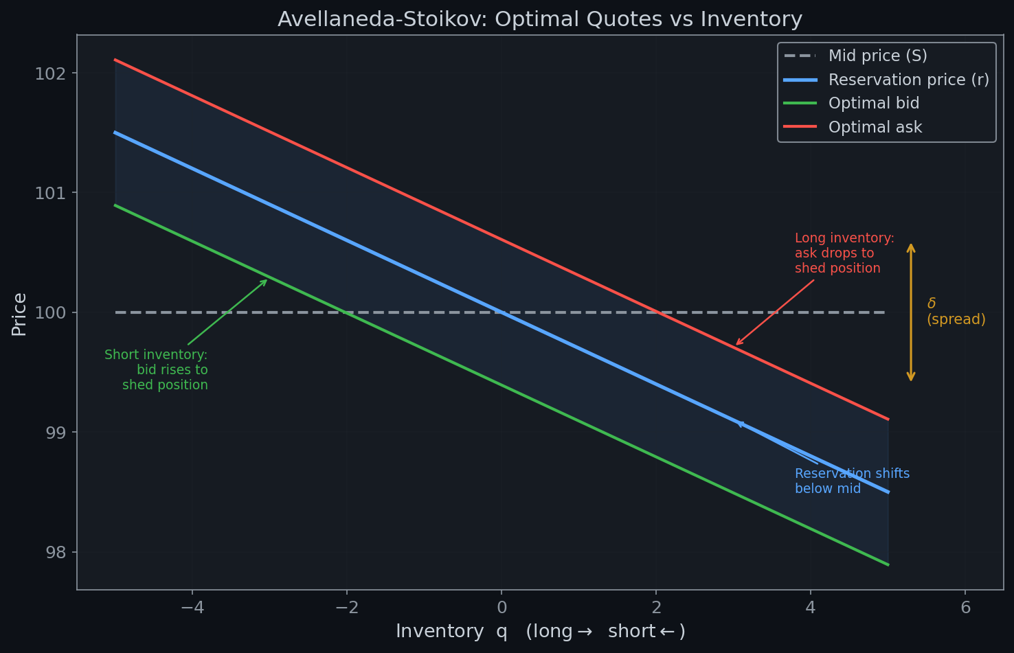
Four lines plotted against inventory (x-axis from long to short):
Mid price: Flat horizontal line
Reservation price: Slopes downward — the MM's internal fair value shifts against inventory
Optimal bid: Below reservation price, slopes down
Optimal ask: Above reservation price, slopes down
As inventory grows long, the MM lowers the ask (to attract sellers) and raises the bid (to discourage buyers). The quotes skew to shed inventory.
The Key Formulas
Reservation price = S − γ · q · σ²(T−t)
Optimal half-spread = (1/γ) · ln(1 + γ/κ)
where γ = risk aversion, q = inventory, σ = volatility, κ = order arrival intensity.
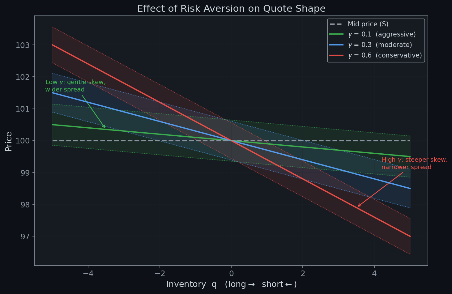
Risk aversion γ controls two things at once: slope (how aggressively the reservation price shifts with inventory) and spread width (how far bid/ask sit from the reservation price). A conservative MM (high γ) skews hard but quotes tight around the skewed level. An aggressive MM (low γ) barely skews but demands a wider spread to compensate.
The Non-Linear Version
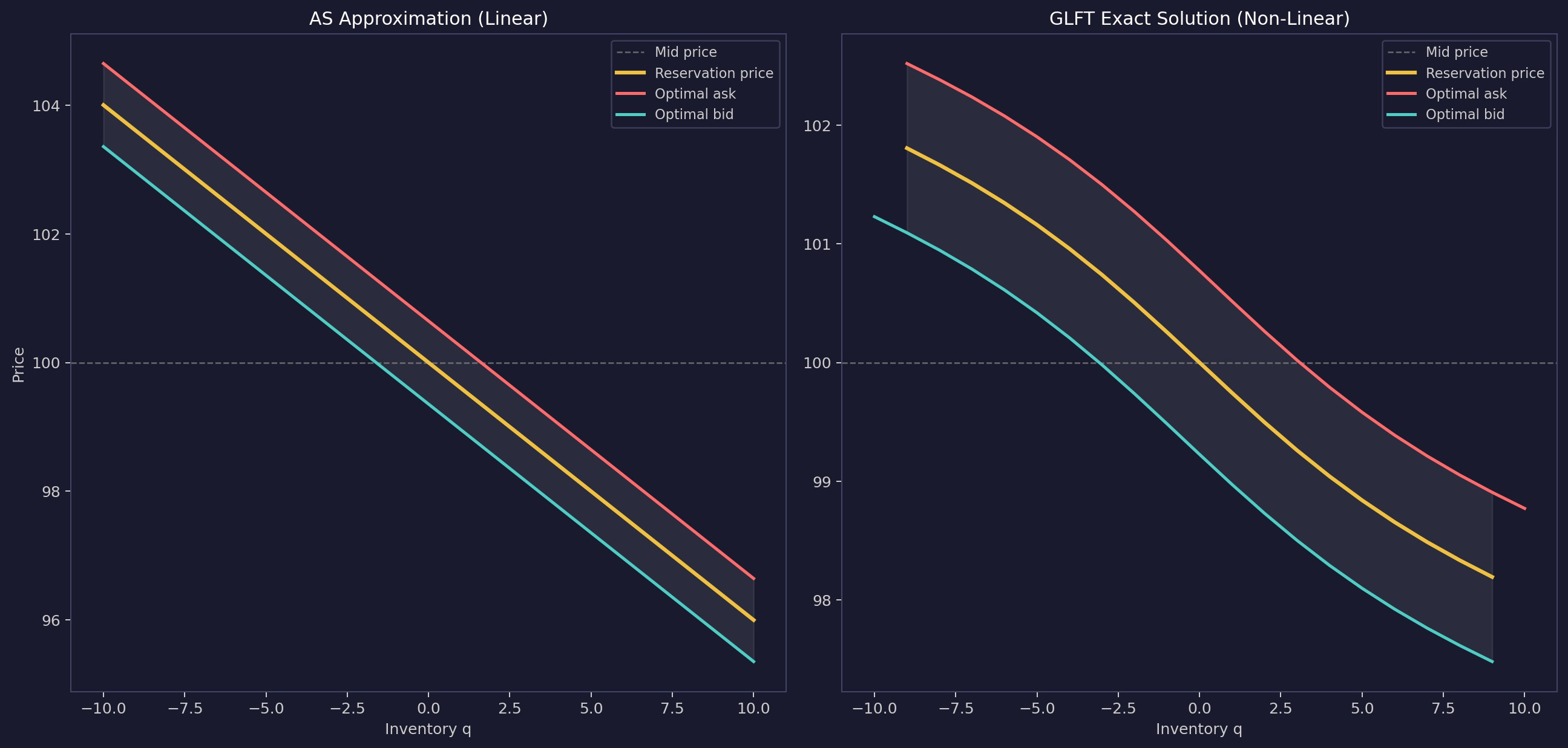
The formulas above are the closed-form approximation. The reservation price is linear in q, the half-spread ignores inventory entirely, and the bid/ask shift in parallel. This is the version everyone cites. But it is not the exact solution.
Guéant, Lehalle & Fernandez-Tapia (2013) solve the full HJB without approximation. The optimal bid and ask offsets from mid become:
δₐ(q) = 1/κ + (1/γ) · ln(ω(q) / ω(q+1))
δ₂(q) = 1/κ + (1/γ) · ln(ω(q) / ω(q−1))
Here ω(q) is the value function at each inventory level, solved from a coupled system of ODEs. Same structure as before: a base spread 1/κ plus a skew term. But the skew now depends on ratios of ω at adjacent inventory levels, not a fixed constant.
When ω is log-linear in q, the log-ratio is constant and you recover AS. In the exact solution, ω curves. The log-ratio grows with |q|:
The skew intensifies at extreme inventory. A position of 10 costs more than twice a position of 5.
The spread widens with inventory. The MM does not just shift quotes, it also becomes less willing to trade on both sides.
Near zero inventory the two models are almost identical. The non-linearity only matters in the tails.
The bid and ask curves bend away from mid more steeply as |q| increases. The reservation price becomes an S-curve around zero rather than a straight line.
In practice you always use the non-linear version, or something equivalent like a quadratic inventory penalty. The linear model tells you that quotes should skew against inventory. The non-linear model tells you how much harder to skew when you are already deep in a position.